How to use Data Modeling for creating Pivot Table in Microsoft excel?

You can use Data Modeling for creating Pivot Table as follows:-

After creating relationships between tables, make use of the data for analysis.

• Click any cell on the worksheet
• Click Insert > PivotTable

• In the Create PivotTable dialog box, under Choose the data that you want to analyze, click Use an external data source

• Click Choose Connection.
• On the Tables tab, in This Workbook Data Model, select Tables in Workbook Data Model.

• Click Open, and then click OK to show a Field List containing all the tables in the Data Model.

Before you can create a PivotTable, you'll need some data. Let's get some sales data from the sample database you downloaded.

1. Download sample data (ContosoV2) for this tutorial. See Get sample data for DAX and Data Model tutorials for details. Extract and save the data files in a location that’s easily accessible, such as Downloads or My Documents.

2. In Excel, open a blank workbook.

3. Click Data > Get External Data > From Access.

4. Go to the folder that contains the sample data files and select ContosoSales.

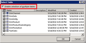
5. Click Open. Because you are connecting to a database file that contains multiple tables, the Select Table dialog appears so that you can choose which tables to import.

   

6. In Select Table, check Enable selection of multiple tables.

7. Choose all of the tables and click OK.

8. In Import Data, click PivotTable Report and click OK.

What happened?

You might not have realized it yet, but you’ve just created a data model. It's created automatically when you import or work with multiple tables simultaneously in the same PivotTable report. The model is mostly transparent in Excel, but you can view and modify it directly using the Power Pivot add-in. In Excel, the presence of a data model is evident when you see a collection of tables in the PivotTable Fields list. There are several ways to create a model. See Create a Data Model in Excel for details.

Exploring data is easy when you drag fields to the Values, Columns, and Rows areas on the PivotTable field list.

1. In the field list, scroll down until you find the FactSales table.

2. Click SalesAmount. Because this data is numeric, Excel automatically places SalesAmount in the Values area.

3. In DimDate, drag CalendarYear to Columns.

4. In DimProductSubcategory, drag ProductSubcategoryName to Rows.

5. In DimProduct, drag BrandName to Rows, placing it beneath subcategory.

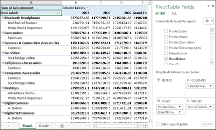
Your PivotTable should look similar to the following screen.

With minimal effort, you now have a basic PivotTable that includes fields from four different tables. What made this task so simple were the pre-existing relationships among the tables. Because table relationships existed in the source, and because you imported all the tables in a single operation, Excel could recreate those relationships in the model.

But what if your data originates from different sources, or is imported at a later time? Typically, you can incorporate new data by creating relationships based on matching columns. In the next step, you’ll import additional tables and learn the requirements and steps for creating new relationships.

Learning how to set up table relationships requires that you have some additional, unconnected tables to work with. In this step, you’ll get the remaining data used in this tutorial by importing one additional database file and pasting data from two other workbooks.

Add product categories

1. In the workbook open a new sheet. You’ll use it to store additional data.

2. Click Data > Get External Data > From Access.

3. Go to the folder that contains the sample data files and select ProductCategories. Click Open.

4. In Import Data, select Table, and click OK.

Add geography data

1. Insert another sheet.

2. From the sample data files, open Geography.xlsx, place the cursor in A1, and then press Ctrl-Shift-End to select all of the data.

3. Copy the data to the clipboard.

4. Paste the data into the empty sheet you just added.

5. Click Format as Table, choosing any style. Formatting the data as a table lets you name it, which will come in handy when you define relationships in a later step.

6. In Format As Table, verify that My table has headers is selected. Click OK.

7. Name the table Geography. In Table Tools > Design, type Geography in Table Name.

8. Close Geography.xlsx to clear it from your workspace.

Add store data

• Repeat the previous steps for the Stores.xlsx file, pasting its contents into an empty sheet. Name the table Stores.

You should now have four sheets. Sheet1 contains the PivotTable, Sheet2 contains ProductCategories, Sheet3 contains Geography, and Sheet4 contains Stores. Because you took the time to name each table, the next step, creating relationships, will be much simpler.

You can immediately begin using fields from the tables you just imported. If Excel cannot determine how to incorporate a field into the PivotTable report, you’ll be asked to create a table relationship that associates the new table with one that is already part of the model.

1. At the top of PivotTable Fields, click All to view the complete list of available tables.

2. Scroll to the bottom of the list. That’s where you’ll find the new tables you just added.

3. Expand Stores.

4. Drag StoreName to the Filters area.

5. Notice that Excel prompts you to create a relationship. This notification occurs because you’ve used fields from a table that is unrelated to the model.

6. Click Create to open the Create Relationship dialog.

7. In Table, choose FactSales. In the sample data you’re using, FactSales contains detailed sales and cost information about Contoso’s business, as well as keys to other tables, including store codes that are also present in the Stores.xlsx file you imported in the previous step.

8. In Column (Foreign), choose StoreKey.

9. In Related Table, choose Stores.

10. In Related Column (Primary), choose StoreKey.

11. Click OK.

Behind the scenes, Excel is building a Data Model that can be used throughout the workbook in any number of PivotTables, PivotCharts, or Power View reports. Fundamental to this model are table relationships that determine navigation and calculation paths used in a PivotTable report. In the next task, you’ll create relationships manually to connect the data you just imported.

Data Model feature allows you to relate multiple Excel tables together and then build Pivot Tables from the related tables. Using this approach, you can effectively build a PivotTable from multiple Excel-based data sources, as long as you maintain those sources as tables. In this tip, you will learn just how easy it is to build a PivotTable using Excel’s Data Model feature. 

CREATING THE DATA MODEL

Before you can build a PivotTable from multiple tables, you must first add the tables to the Data Model. To do so, first ensure that each of the data sources you wish to include in your PivotTable is stored in Excel as a table; if not, convert each data range to a table by clicking in the data range and then choosing Format Format Format Format as Table from the Home tab of the Ribbon. Next, click on any cell in any one of the tables in the workbook and choose PivotTable from the Insert tab of the Ribbon to open the Create PivotTable dialogbox pictured in Figure 1. In the Create PivotTable dialog box, check the box near the bottom of the window labeled Add this data to the Data Model; doing so causes Excel to add all tables in the workbook to the Data Model. Click OK to close the Create PivotTable dialog box.

Figure 1 - Creating a Data Model from a Table in Excel

ESTABLISHING RELATIONSHIPS

Upon closing the Create PivotTable dialog box, Excel displays a window similar to that pictured in Figure 2. Clicking All in the PivotTable Field List causes Excel to show all of the tables included in the Data Model. In the example shown, two tables exist in the Data Model – Product and Trans. The horizontal line drawn between the two tables indicates that these tables are not related. Relating the tables together “joins” them based on the presence of a common field (column) that resides in each table.

Figure 2 - Basic PivotTable Construction Window in Excel

To relate two tables together, click Relationships from the PivotTable Tools Analyze tab of the Ribbon to open the Manage Relationships dialog box. In the Manage Relationships dialog box, click New to open theCreate Relationships dialog box. In the Create Relationships dialog box, select the tables you want to relate together on the left side of the dialog box and the common fields that exist between the two tables on the right side of the dialog box. Figure 3 depicts this process. Click OK to complete the process of relating the tables.

Figure 3 - Creating Relationships between Two Tables

BUILDING A PIVOT TABLE

With the tables related, the process of building the PivotTable is virtually identical to that of building a PivotTable from a non-related, single data source. For example, dragging the Product Name field from the Product table to the Row quadrant, the Customer Name field from the Trans table also to the Row Quadrant, the Year field from the Trans table to the Columns quadrant, and the calc Extension field from the Trans table to the Values quadrant produced the PivotTable pictured in Figure 4. Once constructed, you can manipulate a Pivot Table build from a data model using the same techniques you would use for any other PivotTable.

Figure 4 - PivotTable Constructed from the Data Model

Best Regards , 

SHAMEEM

Exploring data is easy when you drag fields to the Values, Columns, and Rows areas on the PivotTable field list.

1. In the field list, scroll down until you find the FactSales table.

2. Click SalesAmount. Because this data is numeric, Excel automatically places SalesAmount in the Values area.

3. In DimDate, drag CalendarYear to Columns.

4. In DimProductSubcategory, drag ProductSubcategoryName to Rows.

5. In DimProduct, drag BrandName to Rows, placing it beneath subcategory.

Your PivotTable should look similar to the following screen.

With minimal effort, you now have a basic PivotTable that includes fields from four different tables. What made this task so simple were the pre-existing relationships among the tables. Because table relationships existed in the source, and because you imported all the tables in a single operation, Excel could recreate those relationships in the model.

But what if your data originates from different sources, or is imported at a later time? Typically, you can incorporate new data by creating relationships based on matching columns. In the next step, you’ll import additional tables and learn the requirements and steps for creating new relationships.

basm allah alrahman alrahim

great answers , from great people

Create a Data Model in Excel

A Data Model is a new approach for integrating data from multiple tables, effectively building a relational data source inside an Excel workbook. Within Excel, Data Models are used transparently, providing tabular data used in PivotTables, PivotCharts, and Power View reports.

When importing relational data, creating a model occurs automatically when you select multiple tables:

1. In Excel, use Data > Get External Data to import data from Access or another relational database that contains multiple related tables.

2. Excel prompts you to select a table. Check Enable selection of multiple tables.

3. Select two or more tables, click Next, and Finish.

4. In Import Data, choose the data visualization option you want, such as a PivotTable in a new sheet, and build your report.

You now have a Data Model that contains all of the tables you imported. Because you selected the PivotTable report option, the model is represented in the Field List that you’ll use to build the PivotTable report.

What can you do with this model? You can use it to create PivotTables, PivotCharts, and Power View reports in the same workbook. You can modify it by adding or removing tables, and if you use the Power Pivot add-in, you can extend the model by adding calculated columns, calculated fields, hierarchies, and KPIs.

When creating a Data Model, the visualization option is important. You want to choose PivotTable Report, PivotChart, or Power View Report for data visualization. These options allow you to work with all of the tables collectively. Had you chosen Table instead, each imported table would be placed into a separate sheet. In this arrangement, the tables can be used individually, but using all of the tables together requires a PivotTable, PivotChart, or Power View report.

Tip:  Your workbook has data, but do you know whether it contains a Data Model? You can quickly determine model status by opening the Power Pivot window. If data appears in the tabs, a model exists. More about...

Find out which data sources are used in a workbook data model

As you work with a PivotTable and other data visualizations over time, you might lose track of which tables and data sources were added to the data model.

Here are a few easy steps you can follow to determine exactly what data exists in the model.

1. In Excel, click Power Pivot > Manage to open the Power Pivot window.

2. View the tabs in the Power Pivot window.

   Each tab contains a table in your model. Columns in each table appear as fields in a PivotTable Field List. A column that is grayed out has been hidden from client applications.

   

3. To view the origin of the table, click Table Properties.

   If Table Properties is grayed out and the tab contains a link icon indicating a linked table, the data originates from a sheet in the workbook rather than an external data source.

   For all other types of data, the Edit Table Properties dialog shows the connection name and query used to retrieve the data. Make a note of the connection name, and then use Connection Manager in Excel to determine the network resource and database used in the connection:

   1. In Excel, click Data > Connections.

   2. Select the connection used to populate the table in your model.

   3. Click Properties > Definition to view the connection string.

Create a Data Model by importing several related tables.

Click Power Pivot  then  Manage to open the Power Pivot window.

Select a table and apply optimizations: Click Advanced then Default Field Set.

Repeat for other tables.

In Excel, click Insert then select Power View to start a new report.

Thanks for the invitations, full agree with the previous answers , they gave as really a complete lessons.

agree with experts.... Nice answers !

I agree with the previous answers

I agree with M's Ghada and experts answers, thanks for the invitation. .....